Design a Key Value Store

Overview

• A key-value store (key-value database) is a non-relational database
• Unique identifier keys can be plain text or hashed value
• Short keys are more performant than longer keys
• Values can be strings, lists, or objects, etc
• Values are usually treated as opaque objects in Amazon Dynamo DB, Memcached, Redis. (Opaque objects are not coded to interfaces)
• Key-value stores support the following operations:
  • put(key, value)
  • get(key)

Scope

• Keep key size small: less than 10 KB
• Large storage capacity
• High availability
• Automatic scaling (add / remove servers)
• Tunable consistency
• Low latency

Single server architecture

• A single server key-value store can be implemented with an in memory hash map
• Optimization:
  • Compress data
  • Keep frequently used data in memory and store the rest on disc
• A single server key-value store cannot be scaled to support big data

Distributed architecture

• A distributed key-value store is also called a distributed hash table

CAP theorem & distributed systems

According to the CAP Theorem, a distributed system can only achieve two of the following properties:

• Consistency: all clients see the same data no matter which node the connect to
• Availability: all clients get a response even if some nodes are down
• Partition Tolerance: system continues to operate even if two nodes can’t communicate

• CP: (Bank of America)
  • ✅ Consistency: we must block requests until consistency is achieved
  • ✅ Partition tolerance
  • ❌ Availability
• AP: (Twitter)
  • ❌ Consistency
  • ✅ Partition tolerance
  • ✅ Availability: we may return out of data data
• CA: (Not Possible)
  • ✅ Consistency
  • ❌ Partition tolerance
    • Since distributed systems experience network failure, they must support partition tolerance. A CA system cannot exist in the real world
  • ✅ Availability

System Design

Data partition

• Requirements:
  • Data needs to be evenly distributed amongst the available servers
  • Data movements need to be minimized when adding or removing servers
• Method:
  • Consistent hashing
    • meets the requirements specified above
    • the number of virtual nodes per server function as weights to achieve desired loadings. More virtual nodes are assigned to larger servers and fewer virtual nodes are assigned to smaller servers
    • servers can be added or remove`d with minimal impact to data residing in other servers

Data replication

• When we use Consistent hashing, keys and radial locations on the hash ring are generated with a hash function. When the number of nodes are large enough, the server locations are evenly distributed on the circumference of the hash ring. In the diagram below, we see that servers S0, S1 and S3 are bunched together, which results in server S0 receiving more data that the other servers. Whenever a key is mapped to the ring, the algorithm walks clockwise along the ring and added the data to the first server that it finds.

In order to even out the distribution of servers on the circumference of the hash ring, we add virtual server nodes as shown below. (In practice you need hundreds of nodes to achieve standard deviations below 10%. See reference 1)

Let’s say that we have three identical servers and we represent each server with three virtual nodes. Since the locations of servers are generated by a hash function, virtual nodes for different servers are even distributed across the radius of the hash ring.

In order to partition data across a configurable number of servers N, we need to walk along the hash ring clockwise and add data to nodes that correspond to N unique servers. In the diagram below, N = 3 , so we add data for key 4 to server 1 S12, server 2 S22, we skip the next two virtual nodes and then add data to server 0 S02.

In large systems, servers may be located in different geographic regions for better reliability and redundancy.

Consistency

• When data is replicated across multiple nodes, it must be synchronized to ensure consistency
• Definitions:
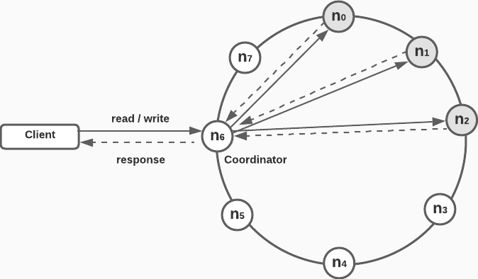
  • N = Number of replicas
  • W = Write quorum. Number of replicas that need to acknowledge a write in order for it to be successful
  • R = Read quorum. Number of replicas that need to respond before a read can be returned successfully
  • The Coordinator is the proxy between the client and the nodes

Tuning consistency parameters:

• Strong consistency guaranteed: W + R > N
• Strong consistency not guaranteed: W + R ≤ N
• Fast Reads: R = 1 and W = N
• Fast Writes: R = N and W = 1

Consistency models:

• Strong consistency: client never sees obsolete data
  • usually achieved by preventing replicas from accepting new read/write operations until the current write is agreed upon by all replicas
  • not ideal for highly available systems (due to blocking)
• Weak consistency: client may see obsolete data
• Eventual consistency: special case of weak consistency where updates propagate and states converge given enough time
  • employed by Amazon Dynamo DB, Cassandra, etc
  • recommended for our system
  • concurrent writes can give rise to inconsistent values in the system, making it necessary for client code needs to reconcile the differences

Inconsistency resolution: versioning

• Replication makes systems highly available but causes inconsistencies
• Versioning & vector clocks can be used to resolve inconsistencies

Vector clocks review

Ruleset:

• Process counters are initialized to zero (0,0,0)
• When a process P1 send a message, it increments its counter and sends the updated time array to the other process, i.e. (1,0,0)
• When a process P2 receives a message, it updates its time array with element-wise maximum of the the incoming array and its own. It finally increments it’s counter by one, i.e. (1, 1, 0)

Vector clock properties

• X is an ancestor of Y if all X ≤ Y element-wise
  • i.e. X=(1,2) < Y=(1,3)
• X is a sibling of Y if any element of Y is less than X
  • i.e. X=(1,2); Y=(1,1)
  • Y[1] < X[1]

Resolving inconsistencies

1. Server 1:
   • var = D1
   • vector clock = (1, 0, 0)
     • P1 += 1
2. Server 1:
   • var = D2
   • vector clock = (2, 0, 0)
     • P1 += 1
3. Server 2:
   • var = D3
   • vector clock = (2, 1, 0)
     • P2 += 1
4. Server 3:
   • var = D4
   • vector clock = (2, 0, 1)
     • P3 += 1
5. Client resolves (assume results sent to S1):
   • var = D1
   • vector clock = (3, 1, 1)
     • P1 += 1

Downsides

• Vector clocks are complex and require client logic to resolve conflicts
• Server-version data can become large. To solve this problem, a threshold is set to drop old data. This introduces inefficiencies in resolution, but has proven an acceptable solution in Amazon DB

Handling failures

• Failures occur commonly in distributed systems
• Since components of distributed systems are unreliable, a server cannot be classified as down just because another server believes that it is. The Gossip protocol is commonly used to classify offline servers

Gossip protocol

• Each node maintains a node members list that keeps track of member_ids and heartbeat counters
• Each note periodically updates its heartbeat counter
• Each note periodically sends heartbeats to random nodes, which in turn promulgates (officially announces) its status to another set of random nodes
• Each Node update their membership lists when they receive official heartbeat announcements from other nodes
• If the heartbeat counter for a node has not been updated in a specified period of time, the node is classified as offline

Handling temporary failures

• Strict quorum approach: read/write operations could be blocked
• Sloppy quorum approach: improves availability by choosing the first W healthy servers for writes (on the hash ring) and the first R healthy servers for reads. Offline servers are ignored. When servers come back online, changes can be pushed to the newly started server using a process called hinted handoff. (Hinted handoff is a method that allows another node to accepts writes on behalf of an offline node. The data is kept in a temporary buffer and is written back to the other node once it is restored to service. This is how Dynamo DB accomplishes it “Always writable” guarantee)

Handling permanent failures

• If a replica goes offline permanently, hinted handoff won’t help us. To address this situation, we implement an anti-entrophy protocol to keep replicas in sync. Anti-entropy compares each piece of data in the replicas and updates each replica with the latest version.

Merkle Trees can be used to efficiently detect differences in replicated data structures. A Merkle tree is a binary tree whose leaf nodes are the hashes of portions of the data, and whose internal nodes are hashes of the children node hashes.

Creating a Merkle tree

1. Divide the keyspace into buckets (4 in the diagram below)
2. Hash each key in each bucket
3. Create a single hash per bucket
4. Build the Merkle tree by calculating node hashes from the children hashes

Detecting data inconsistencies

• If the root hashes are different, we know that the two servers are not in sync with each other. By traversing the left and then the right branches, the bucket(s) that are out of sync can be efficiently located and reconciled
• Using a Merkle tree, the subset of data that needs to be synchronized is dramatically smaller than the total amount of data stored
• A large production system that had 1 billion keys could have 1 million buckets with 1 thousand keys each. If the data for one of the keys was out of sync, the bad bucket could be found by traversing the binary tree. Only 1000 keys would need to be updated
• In real-world systems, power outages, network outages, natural disasters, etc can take entire data centers offline. In situations like this, its important for data to be replicated across geographically diverse data centers. If one data center goes down, the replicas can continue to serve customers

System architecture diagram

• Client sends get(key) / put(key, val)requests to the key-value store via an API
• The coordinator acts as the proxy between the client and the distributed system
• Server nodes are more or less evenly distributed along the hash ring
• The system is decentralized as nodes and be automatically added and removed
• Data is replicated over several data centers and does not have a single point of failure

System diagram

Node diagram

• Since the design is decentralized, each node performs many different functions
  flowchart LR subgraph Node A[Client API] B[Failure detection] C[Conflict resolution] D[Failure repair] E[Storage engine] F[etc] end

Write path

1. Persist write request to disk
2. Add memory to in-memory cache (hash map)
3. Flush data to SSTables when the cache reaches is full or it reaches predefined thresholds. An SSTable (sorted string table is a sorted list of <key, value> pairs)

Read path (data in memory)

• If the data is cached in memory, result is retrieved and returned

Read path (data on disk)

1. Check if data is cached in memory, return it if it is
2. If the data is not cached in memory, the Bloom filter efficiently finds out which table the data is stored in
3. Using location information from the Bloom filter, the results data is returned to the client

Source

1. System Design Interview by Alex Xu
2. Grokking the Advanced System Design Interview